Grabbing electronic data from public sources is all very well, but what about processing and analytics? Any data type will succumb to analysis, pictures, sounds – you name it – but for now we will stick with numbers & words. And because it is not something that investors do every day, we’ll focus on the words first.
Dumb Computers
When parsing text (linguistic information if we want to get fancy) using a data harvest the raw material returns as textstrings.Those characters have no meaning, knowledge or information as far as the computer is concerned; they’re just a visual representation of stored binary code.
Encodings Sidebar
There’s an important topic regarding text encoding and its handling – these types of errors trip all of us up from time to time, crashing our otherwise smoothly-running scripts – but we will set this rather-dry theme aside for now, returning to in a later post.
HTML –> Raw –> Text
By its very nature, parsing gets rid of the excess html (tags, structure, formatting and the like) but you are still left with material that can be quite raw (e.g excess whitespace, line breaks, blank lines etc.) and needs further pre-processing.
We convert that raw string into text via tokenization (again, a fancy way to say “break into word tokens”). There are design choices about that process (e.g should £4.22 be split four ways?) but, give or take, words exist between whitespaces.
Our first Bag of Words
So we’ve got our bond prospectus in usable format (handily translated of course, see PDF is Evil!), we convert it to text, and then we can run any analysis we choose. We’ll use the brilliant nltk package in the code below, but there are many others to choose from, or, in truth, we could have performed ourselves without any imports using a .split(‘ ‘) method.
import nltk toks = nltk.wordpunct_tokenize(raw) text = nltk.Text(toks) |
With our bag of words in token form let’s give this one last clean, lower-casing everything, getting rid of stop-words (‘i’, ‘we’, ‘up’, ‘in’ etc.), complicating affixes and ensuring our stem-words sit in dictionaries (lemmatisation). There are of course variants, but this approach will suffice. Here’s that all wrapped-up in a quick definition –
def processraw(text): 'final clean-up of text' text = [t for t in text if t.lower() not in stopwords] # lowercase, non-stopwords text = [wnl.lemmatize(t) for t in text] # wordnet lemmatizing return [t for t in text if t.isalnum()] # only give alphanumerics |
Quick & Dirty Analysis
Obviously we can instantly calculate document stats (character counts, words, sentences, vocabulary, keywords etc. – see below), but that only takes you so far.
Similarly, using the underlying text we can actively search* for the usage of certain expressions or phrases:
– generating the contexts in which it is used (concordance);
– finding other words used in similar contexts;
– we can pair our similarity-words above to find common contexts; or
– we can develop n-grams (n words appearing next to one another) (collocations).
*Of course we can beef up Search using Regular Expressions (Regex), but that’s for another post.
Again, you get the idea; it’s a bit more useful, but not terribly dramatic. Let’s change gears.
Internal Structure
Semantically-oriented dictionaries hold words as well as word relationships (think of a sophisticated and interactive dictionary + thesaurus), and one of these is WordNet (developed at Princeton).
The building block of WordNet might be described as the ‘synset’ (a set of synonymous words), each of which holds a definition and from which we can draw examples (think of the synset as a bag with an idea inside it).
So, for example, the term ‘credit’ sits in more than 10 synsets; each of which captures ideas such as ‘give someone credit for something’, ‘have trust in; trust in the truth or veracity of’, ‘ascribe an achievement to’ etc.
Each synset (c. 120,000 total) sits within an abstract concept hierarchy, with synsets becoming less/more specific as you travel up/down the chain to generate lexical relations. So for example we can generate hypernyms (a synset’s more abstract parents) and hyponyms (our synset’s more-specific children), as well as many other metrics.
So for example: where ‘credit’ captures the idea of ‘have trust in; trust in the truth or veracity of’ the pathway is as follows:
Synset(‘think.v.03’) —> Synset(‘evaluate.v.02’) —> Synset(‘accept.v.01’) —> Synset(‘believe.v.01’) —> Synset(‘trust.v.01’) —> Synset(‘credit.v.04’)
It’s early days, but hopefully you’re beginning to see how this type of analysis can, with a little work, become more significant, and that we are taking our first tentative steps on the road to inference.
Skim-Reading (robot-style)
Let’s get practical. Here’s how we might apply some of the above – let’s skim-read, robot-style.
Our robot quickly (very quickly!) read our prospectus (green) and began making mental comparisons to other documents (orange). We do this by memory and lookup; the robot did it by contra-reading a whole catalogue of documents.
That catalogue (referred to as a Corpus) forms the robot’s background knowledge. So choose it carefully (or very widely). We read in a million words (it says half a mill below but that count excludes stopwords) from the well-established Brown Corpus which covers a wide range of topics.
Let’s look at the graphics below (too many words here!) and then I’ll provide some explanations below –
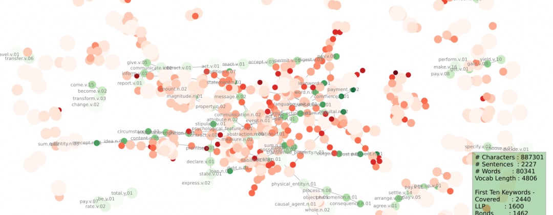

What’s going on?
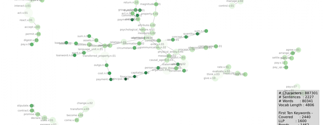
Starting with the green-only graph: we’re trying to visually capture the ideas contained within our prospectus.
We took all the keywords in each doc, found each of their synsets, and then found each synset’s pathways from its root (there can be many), counted them up and kept the important (oft-repeated) ones. We draw those tramlines connecting our specific/concentrated keyword ideas (small dark-dots) up to their parents (pale, diffuse dots).
Notice how these results are distinctly different to the keywords. Nice.
Mixed Graphs
These graphs (they’re the same, one just has labels switched off) map the overlap that our robot sees as it compares our document (prospectus, greens) with a universe (Brown Corpus, orange).
That overlap represents the specificity of our text (what it’s about, and also what it’s not about). It’s the robot’s version of first impressions, or skim-reading, as we said above.
Next Steps
We’ve come a long long way from keywords, but let’s not kid ourselves, we are not yet at enlightenment (patience, young grasshopper!). Despair not, this is only an introductory blog – we’ve only just scratched the surface.
Similarity testing, Sentiment Analysis, Text Summarisation, Latent Semantic Analysis and more, all lie ahead of us…